Getting Started
The RoGaTa engine builds upon `Ros Noetic`_ to interface with the robots, and OpenCV-Python to calibrate the arena and track all dynamic objects. The first step is thus to install ROS on all robots as well as the host PC.
The host PC refers in this case to the PC which runs the engine which means that additionally OpenCV has to be installed there.
Setting up the Environment
Once ROS and OpenCV are installed the environment of the engine has to be set up. First, a catkin workspace has to be created. For this catkin tutorial can be followed.
The RoGaTa Engine itself is a ROS package containing nodes for camera-based sensing and a library that provides utilities for game development.
The package has to be placed inside the catkin_ws/src directory:
cd ~/catkin_ws/src
git clone https://github.com/liquidcronos/RoGaTa-Engine
Afterward, the catkin_make command has to be called inside the catkin_ws directory:
cd ..
catkin_make
If everything is correctly installed, the following command should change the current directory to the one containing the ROS package:
roscd rogata_engine
The package installation should also install the rogata_library, a python package which allows for writing of of own game objects and extensions to the engine.It is imported by calling
import rogata_library as rgt
Warning
The rogata_library depends on other packages. While catkin_make should automatically resolve them, it does not check for a minimum version.
On old systems this might lead to problems. For this reason the /src directory contains a requirements.txt file that can be used to update all the needed python packages.
This is done by calling sudo pip install -r /path/to/requirements.txt.
Setting up the Game Area
The first step in actually using the engine is to set up the game area.
Since the engine needs a camera to calibrate itself and track at least one rogata_library.dynamic_object, the first step is setting up a camera.
The Camera needs to be affixed above the game area perpendicular to the ground. In General the higher up the camera the better since it leads to a larger game area. However, it also decreases the precision of the object tracking. This also means that bigger markers have to be used. This can of course be circumvented by using a higher resolution camera. Since higher resolution pictures take longer to process this could however slow down the engine depending on the computer it’s running on.
Note
Once the camera is set up, a picture of the game area can be taken. Such a picture can be used as a reference for the size of the game area. This prevents setting up game objects which end up partially outside of the camera view.
After the camera is installed the area itself has to be prepared. Given a desired layout of static objects, color has to be applied to the ground to mark the borders of the object. The easiest way to do this is using colored tape.
The colors of the tape should be chosen to strongly contrast the grounds hue. An example of a prepared game area can be seen below.

Setting up a Scene
Scenes can be thought of as real-life video game levels. A Scene is made up of multiple game objects whose position is determined by a camera above the physical level. Setting up a scene thus simply means getting the engine to recognize physical objects as game objects.
The RoGaTa engine uses a simple recognition based on the color of an object. The full theory behind the detection of game objects can be seen in `How it Works`_.
Calibrating the Arena
To calibrate the arena the calibrate_scene.py script can be used. It is called using:
python calibrate_scene.py PATH_TO_IMAGE
Where PATH_TO_IMAGE is the path to an image of the scene.
This image has to be captured with the same stationary camera used to later track dynamic objects.
The script will open a window where one can see the image of the scene as well as several sliders:
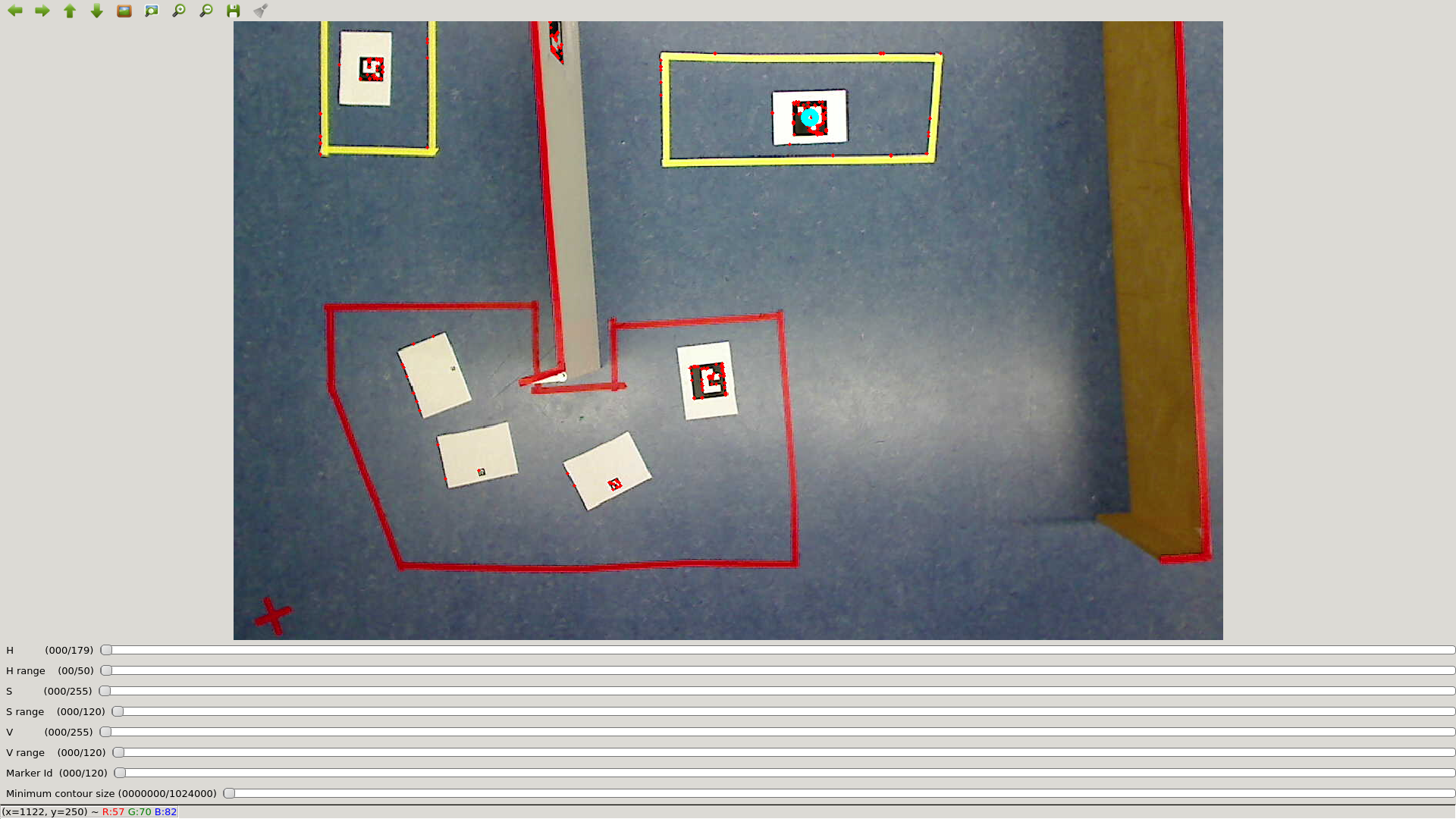
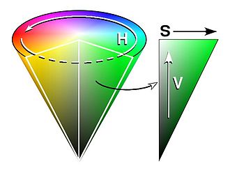
The first six sliders are used to select the color of the desired object. This color is specified in the HSV colorspace. HSV refers to Hue, Saturation, and Value. A good visualization of the HSV values can be seen in this image from its wikipedia page:
For OpenCV, The Hue Range goes from 0-179 (which is half that of the common Hue definition which goes from 0 to 359). since the Hue value is cyclical, both these values represent a type of red. While the borders between colors are not clearly defined the following table gives an idea which hue values to pick for each object color
| Color | Hue Value Range |
|---|---|
| Red | 0-30 |
| Yellow | 31-60 |
| Green | 61-90 |
| Cyan | 91-120 |
| Blue | 121-150 |
| Mageta | 151-179 |
Saturation and Value are defined from 0-255. The less saturated an image, the less colorful it is. Additionally the lower its value, the darker it is.
Due to different lighting conditions across the scene, these last two values will vary for an object. For this reason, each object also has a range slider. Each range d specifies an acceptable color interval of [VALUE-0.5d, VALUE+0.5d] Where VALUE is the value of the main slider.
Note
For fast tuning, it is advisable to first select the desired hue value while setting the saturation and value ranges to the maximum. From there it is easy to dial in the values until the desired object is selected.
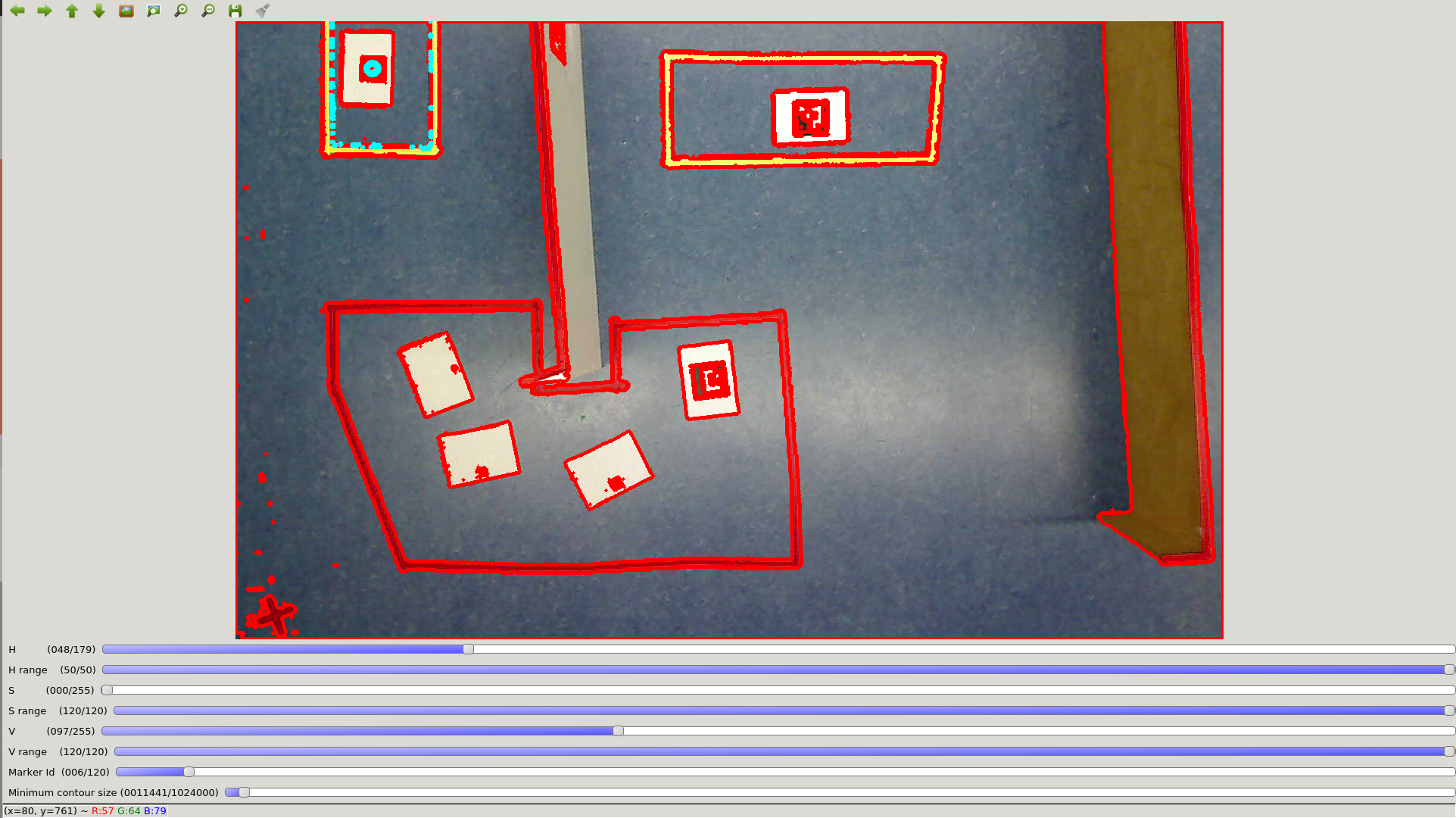
Example values for the sliders can be seen in the following image:
As one can see there are multiple objects outlined in red. To pick the desired object to track, aruco markers are used. If placed inside the desired object, the contour can be selected by specifying the corresponding marker ID using the Marker ID slider.
Note
It is possible to directly specify values by clicking on the slider values on the left
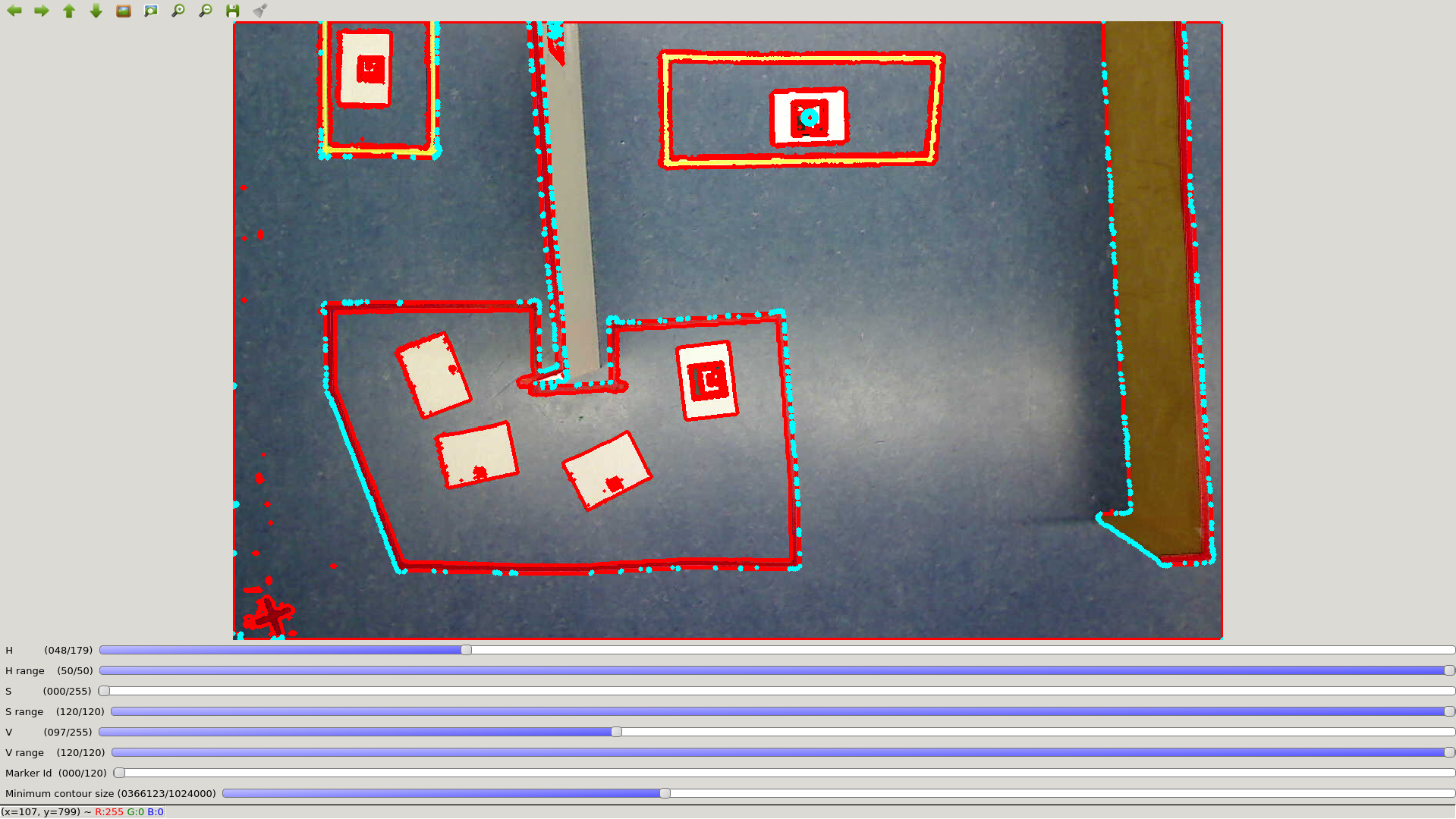
Selecting Marker 1 results in the following image:
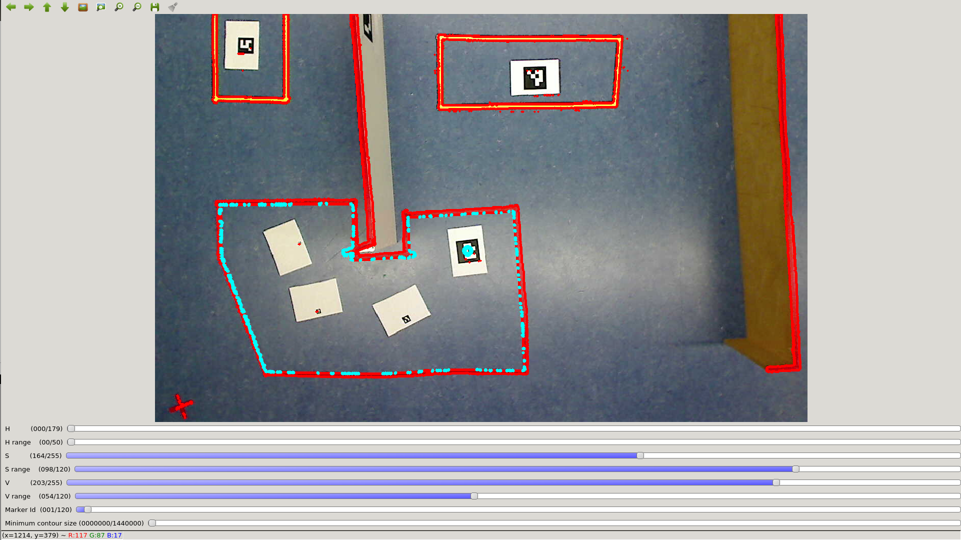
the currently selected contour is now highlighted in torques. It can now be saved by pressing s on the keyboard. The Terminal in which the calibrate_scene.py script was called will now ask for a file name. If provided it saves the contour as a .npy object.
This procedure can now be repeated for each contour.
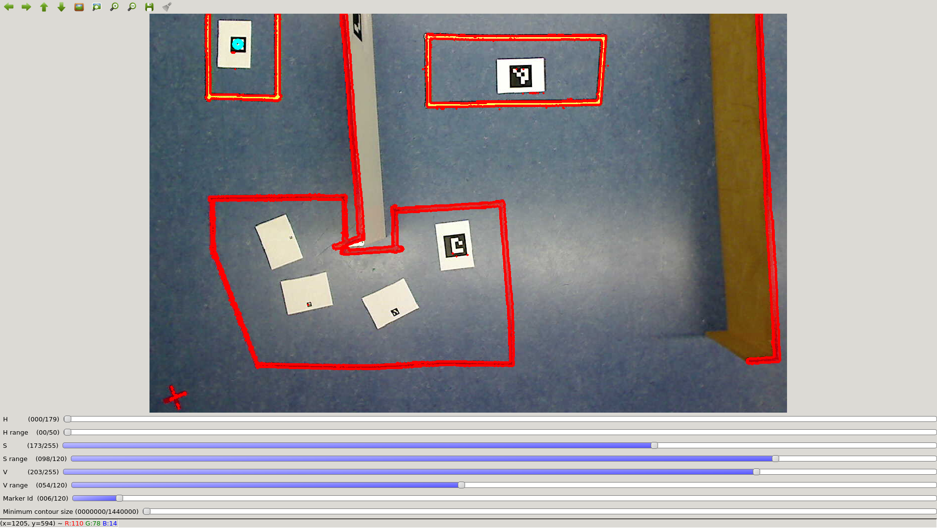
If there are very small objects inside the scene such as walls or open contours such as the yellow one in the top left a trick can be employed. Instead of using the color of the object, the color of the Ground can be used. This specifies a contour around the desired object which can then be selected.
However, in this case, the border of the marker itself might count as a contour. To circumvent this the Minimum Contour Size slider can be used to specify the minimum size of the chosen contour. This way it is possible to select such open object:
However, this trick might also select other game objects such as seen here when specifying the contour of the wall:
This can be circumvented by first setting up the walls and using an image of the arena without the other objects.
Building Game Objects
Using the contours calibrated in the last section it is possible to set up game objects.
The architecture of the game objects is described in the how it works section.
In the above example, the game area has two objects, the yellow goals and the red line of sight breakers
Note
One can of course also have multiple objects of the same color. This is however only advisable if they behave similarly as it might otherwise be confusing when playing or observing a game.
the first step in setting up the objects is loading the contour objects saved by calibrate_scene:
import rogata_library as rgt
import numpy as np

# Setting up the goal object
left_goal  = np.load('left_yellow_rectangle.npy')
right_goal = np.load('right_yellow_rectangle.npy')
goals      = rgt.GameObject('goals',[left_goal,right_goal],np.array([1,1]))


# Setting up the line of sight breakers
large_polygon = np.load('red_polygon.npy')
floor_trick   = np.load('floor.npy')
los_breakers  = rgt.GameObject('line_of_sight_breakers',
                                [large_polygon,floor_trick],
                                np.array([1,-1]))
Setting up the first object is rather straight forward, the contours are loaded and are used to initialize the game object. The object hierachy is [1,1], since both objects are simple objects sitting side by side.
For the line of sight breakers however the floor contour trick was used. Since this mapped the inverse of the red object, so long as one is within the floor contour one is not inside a line of sight breaker. For this reason, the object gets a contour hierarchy of -1.
Warning
This only works because the Floor polygon does not include the large red polygon. If the floor contour was saved before the polygon was drawn, inside the polygon would also register as being outside of the object!
In addition to the static objects on the floor, robots themself also need to be set up as a rogata_library.dynamic object.
Assuming the Robot is equipped with a marker with ID 6, it can be initialized using:
# Setting up the robot object
name      = "pioneer_robot"
id        = 6
hit_box   = {"type":"rectangle","height":30,"width":30}
robot_obj = rgt.dynamic_object(name,hit_box,id)
the hitbox specifies the space the robot takes up in the arena.
For now, this has to be set manually, however, a future script similar to calbibrate_scene.py is planned.
Building a Scene
Using these two objects a scene can now be built witch enables the basic functionalities of the engine. It can be set up using:
example_scene =rgt.scene([goals,los_breakers,robot_obj])
This scene can now be packacked inside a ROS Node:
#!/usr/bin/env python
import numpy as np
import rogata_library as rgt
import rospy


# Setting up the goal object
left_goal  = np.load('left_yellow_rectangle.npy')
right_goal = np.load('right_yellow_rectangle.npy')
goals      = rgt.GameObject('goals',[left_goal,right_goal],np.array([1,1]))


# Setting up the line of sight breakers
large_polygon = np.load('red_polygon.npy')
floor_trick   = np.load('floor.npy')
los_breakers  = rgt.GameObject('line_of_sight_breakers',
                                [large_polygon,floor_trick],
                                np.array([1,-1])


# Setting up the robot object
name      = "pioneer_robot"
id        = 6
hit_box   = {"type":"rectangle","height":30,"width":30}
robot_obj = rgt.dynamic_object(name,hit_box,id)


if __name__ == "__main__":
    try:
        rospy.init_node('rogata_engine')
        example_scene =rgt.scene([goals,los_breakers,robot_obj])
    except rospy.ROSInterruptException:
        pass
The node can be started with:
rosrun PACKAGE_NAME SCRIPT_NAME.py
But in order to be recognized the node first has to be made executable using the following command:
chmod +x SCRIPT_NAME.py
More information about ROS and what a Package is can be found in the ROS tutorials.
It is strongly encouraged that one familiarizes himself with ROS before trying to use the RoGaTa Engine.
If the scene is initialized correctly it should publish the position of the robot and provide a multitude of services. The existence of the publisher can be checked using
rostopic echo /pioneer_robot/odom
Which should return odometry values. The services offered by the engine can be checked using
rosservice list
- These should include:
- set_position
- get_distance
- intersect_line
- check_inside
Tracking Dynamic Objects
The Tracking of dynamic objects, while a game is running, was consciously decoupled from the scene node, because there are multiple approaches suited for different use cases.
If the objects should be tracked with a camera, the :py:function:`rogata_library.track_dynamic_objects` function can be used. Using a grayscale image it can track a list of dynamic objects. To use it with ROS one can use cv_bridge to convert published Images of a camera node into usable images:
#!/usr/bin/env python
import sys
import cv2
import rospy
import rogata_library as rgt
from sensor_msgs.msg import Image
from cv_bridge import CvBridge
import numpy as np


def img_call(ros_img,object_name_list):
    cv_img = bridge.imgmsg_to_cv2(ros_img,'mono8')
        rgt.track_dynamic_objects(cv_img,object_name_list)


if __name__ == '__main__':
    try:
        rospy.init_node("Dynamic Object Tracker")
                bridge       = CvBridge()
                object_numb  = len(sys.argv)
                object_list  = [sys.argv[i] for i in range(2,object_numb)]
        cam_sub      = rospy.Subscriber(sys.argv[1],Image,img_call,object_list)
        rospy.spin()
    except rospy.ROSInterruptException:
        rospy.loginfo("Dynamic Object Tracker  Node not working")
However, it is also possible to use the track_image function on a prerecorded video.
In some cases, however, tracking with a camera is not beneficial.
This is why in general own functions can be written to track such objects. They can then update the Position of the objects using the set_position service.
Using the Engine in Gazebo
One possible for such a scenario would be when using the engine inside a simulation such as Gazebo. While a simulation already provides much of the tools the rogata engine provides it might be beneficial to be able to simulate a given game before implementing it in the real arena.
Scenes can be set up in Gazebo the same way that normal scenes are set up, however instead of a camera the position of dynamic objects is directly provided by the simulation.
Note
For robots this position is usually provided by a Odometry Topic.
However the image used for the setup is in this case not captured by the camera above the scene. Instead an arbitrary image can be used that is then set as the ground texture in Gazebo. A tutorial of how to do this can be found here.
All that remains is to convert the odometry positions of the simulation into pixel position in the game area. Given a specified 2 dimensional scale \(X_{sim}\) in meters in the simulation, and image dimensions \(X_{game}\) in pixels the conversion for a image point \(P_{sim}\) into a point \(P_{game}\) is calculated using:
\(P_{game} = [P_{sim}_{x}, -1*P_{sim}_{y}]* ||X_{game}||/||X_{sim}|| - X_{game}/2\)